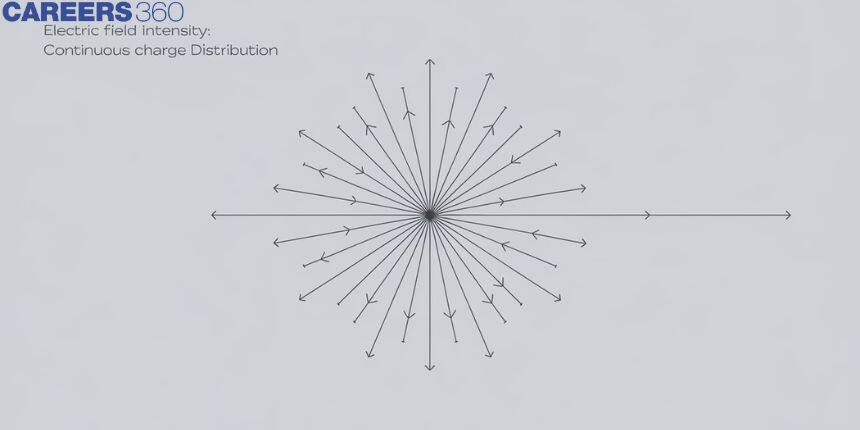
Electric Field Intensity: Continuous Charge Distribution

Electric field and electric lines of force

The space around a charge in which another charged particle experiences a force is said to have an electric field in it.

Electric Field Intensity

The electric field intensity at any point is defined as the force experienced by a unit of positive charge placed at that point.

$
E=\frac{F}{q_0}
$
where F is the force experienced by q 0 . The SI unit of E is,
$
\frac{\text { Newton }}{\text { Columb }}=\frac{\text { Volt }}{\text { meter }}=\frac{\text { Joule }}{\text { Coulomb } \times \text { Meter }}
$

The dimensional formula is $\left[M L T^{-3} A^{-1}\right]$

The electric field is a vector quantity and the positive charge is away from the charge and for the negative charge, it is towards the charge.

What is Discrete charge distribution?

Discrete charge distribution refers to a situation where electric charges are located at distinct, separate points rather than spread out continuously. Each charge creates its own electric field, and the overall effect is determined by the contributions from these individual point charges. This concept is important for understanding how electric forces interact in systems with isolated charged particles or objects.

What is Continuous charge distribution?

An amount of charge distributed uniformly or non-uniformly on a body. It is of three types :

1. Linear charge distribution

$(\lambda)$ - charge per unit length.
$
\lambda=\frac{q}{L}=\frac{C}{m}=C m^{-1}
$

Example: wire, circulating ring

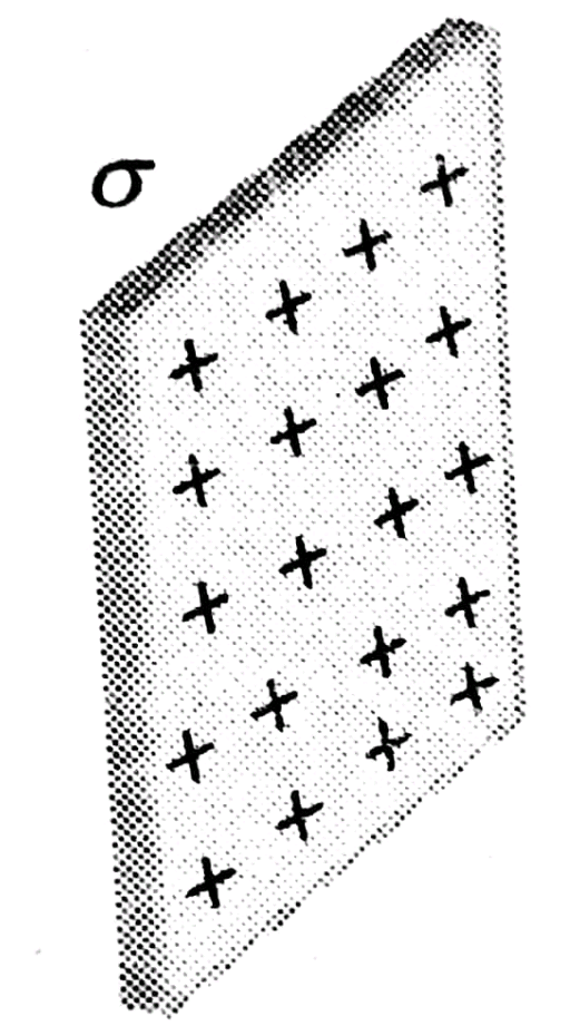
2. Surface charge distribution

$(\sigma)$ - charge per unit Area
$
\sigma=\frac{Q}{A}=\frac{C}{m^2}=C m^{-2}
$

Example: plane sheet

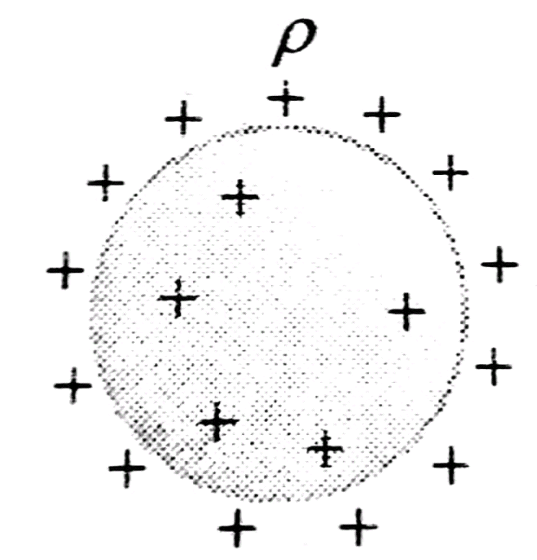
3. Volume Charge distribution

$(\rho)$ - charge per unit volume.
$
\rho=\frac{Q}{V}=\frac{C}{m^3}=C m^{-3}
$



Example - charge on a dielectric sphere etc.

Now we will discuss one example and derivation of the electric field due to a uniformly charged rod.

So, let us consider a rod of length l which has uniformly positive charge per unit length lying on the x-axis, dx is the length of one small section. This rod has a total charge Q and dq is the charge on the dx segment. The charge per unit length of the rod is $\lambda$. We have to calculate the electric field at a point P which is located along the axis of the rod at a distance of 'a' from the nearest end of the rod, as shown in figure

The field $d \vec{E}$ at P due to each segment of charge on the rod is in the negative "x" direction because every segment of the rod carry a positive charge. In this every segment of the rod is producing an electric field in the negative "x" direction, so the sum of the electric field can be added directly and can be integrated because all electric field lies in the same direction.

Now, here $-d q=\lambda \cdot d x$

$
d E=k_{\mathrm{e}} \frac{d q}{x^2}=k_{\mathrm{e}} \frac{\lambda d x}{x^2}
$

The total lield at $P$ is
$
E=\int_a^{l+a} k_e \lambda \frac{d x}{x^2}
$

If $k_e$ and $\lambda=Q / l$ are constants and can be removed from the integral, then
$
\begin{aligned}
& E=k_e \lambda \int_a^{l+a} \frac{d x}{x^2}=k_e \lambda\left[-\frac{1}{x}\right]_a^{l+a} \\
& \Rightarrow k_e \frac{Q}{l}\left(\frac{1}{a}-\frac{1}{l+a}\right)=\frac{k_e Q}{a(l+a)}
\end{aligned}
$

Now if we slide the rod toward the origin and the $a \rightarrow 0$, then due to that end, the electric field is infinite.

Electric field strength due to a charged circular arc at its centre

Let's try to find out the electric field at the centre of an arc of linear charge density $\lambda$, radius R subtending angle $\phi$ at the centre.

If $Q$ is the total charge contained in the arc then,
$
\lambda=\frac{Q}{R \phi}
$

By symmetry, we know that the electric field due to the arc will be radially outward at the centre.

Now consider a small element of the arc of charge
$d Q=\lambda R d \theta$on either side of the horizontal to the arc.

Now resolving the electric field due to the small element of the arc $\lambda R d \theta$,

we see that both the vertical components get canceled and all that remains will be the horizontal component of the electric field due to the corresponding small
elements.

So we have $2 d E \cos \theta$ due to all such corresponding small elements on the arc,

so, by integrating all those electric fields due to these small elements we get the electric field due to the whole arc.

$E=\int_0^{\frac{\phi}{2}} 2 d E \cos \theta .... (1)$.
We know that electricity due to charge dQ is given by,$\begin{aligned} & d E=K \frac{d Q}{R^2} \\ & \text { But, } d Q=\lambda R d \theta \\ & d E=K \frac{\lambda R d \theta}{R^2}=K \frac{\lambda d \theta}{R}\end{aligned} .......(2)$

Substituting (2) in (1)

$\begin{aligned} & E=\int_0^{\frac{\Delta}{2}} 2 K \frac{\lambda \cos \theta d \theta}{R} \\ & \Rightarrow E=\frac{2 K \lambda}{R} \int_0^{\frac{\pi}{2}} \cos \theta d \theta \\ & \Rightarrow E=\frac{2 K \lambda}{}[\sin \theta]_0^{\frac{\theta}{2}} \\ & \Rightarrow E=\frac{2 R \lambda}{R}\left(\sin \left(\frac{\phi}{2}\right)-\sin 0\right) \\ & \Rightarrow E=\frac{2 K \lambda \sin \frac{\Delta}{2}}{R} \\ & \quad K=\frac{1}{4 \pi \varepsilon_0} \\ & \text { Using } \\ & \therefore E=\frac{2 \lambda}{4 \pi \varepsilon_0 R} \sin \frac{\phi}{2}\end{aligned}$

Recommended Topic Video

Solved Examples Based on Electric Field Intensity: Continuous Charge Distribution

Example 1: The electric field inside a spherical shell of uniform surface charge density is

1) Zero

2) Constant, less than zero

3) Directly proportional to the distance from the centre

4) None of the above

Solution:

Surface charge distribution
$(\sigma)$ - charge per unit Area
$
\sigma=\frac{Q}{A}=\frac{C}{m^2}=C m^{-2}
$

wherein

(Plane sheet, sphere, cylinder etc)

All charge resides on the outer surface so that according to Gauss's law, the electric field inside a shell is zero.

Hence, the answer is option (1).

Example 2: The electric field near a conducting surface having a uniform surface charge density $\sigma$ is given by
1) $\frac{\sigma}{\varepsilon_0}$ and is parallel to the surface
2) $\frac{2 \sigma}{\varepsilon_0}$ and is parallel to the surface
3) $\frac{\sigma}{\varepsilon_0}$ and is normal to the surface
4) $\frac{2 \sigma}{\varepsilon_0}$ and is normal to the surface

Solution:

Surface charge distribution

$(\sigma)$ - charge per unit Area
$
\sigma=\frac{Q}{A}=\frac{C}{m^2}=\mathrm{Cm}^{-2}$
The electric field near the conductor surface is given by $\frac{\sigma}{\varepsilon_0}$ and it is perpendicular to the surface.

Hence, the answer is option (3).

Example 3: What is Volume charge distribution for Non conducting charged sphere

1) $\lambda=\frac{Q}{2 \pi R}$
2) $\sigma=\frac{Q}{4 \pi R^2}$
3) $\rho=\frac{Q}{\frac{4}{3} \pi R^3}$
4) none

Solution:

For a non-conducting charged sphere, the volume of the sphere is given by:

$
V = \frac{4}{3} \pi R^3
$

The volume charge density \(\rho\) is defined as the total charge \(Q\) divided by the volume \(V\):

$
\rho = \frac{Q}{\frac{4}{3} \pi R^3}
$

Simplifying the expression:

$
\rho = \frac{3Q}{4 \pi R^3}
$

Thus, the correct expression for the volume charge density \(\rho\) is:

$
\boxed{\rho = \frac{Q}{\frac{4}{3} \pi R^3}}
$

Therefore, the correct option is (3).

Example 4: Charge is distributed within a sphere of radius R with a volume charge density $\rho(r)=\frac{A}{r^2} e^{\frac{-2 r}{a}}$, where A and a are constants. If Q is the total charge of this charge distribution, the radius $R$ is:

1) $\frac{a}{2} \log \left(\frac{1}{1-\frac{Q}{2 \pi a A}}\right)$
2) $\frac{a}{2} \log \left(1-\frac{Q}{2 \pi a A}\right)$
3) $a \log \left(1-\frac{Q}{2 \pi A a}\right)$
4) $a \log \left(\frac{1}{1-\frac{Q}{2 \pi a A}}\right)$

Solution:

Volume Charge distribution
$(\rho)$ - charge per unit volume.
$
\rho=\frac{Q}{V}=\frac{C}{m^3}=C m^{-3}
$

wherein

(charge on a dielectric sphere etc)

$\begin{aligned}
Q & =\int \rho d V \\
& =\int_0^R \frac{A}{r^2} e^{-2 \frac{r}{a}}\left(4 \pi r^2\right) d r \\
& =2 \pi a A\left(1-e^{-2 \frac{R}{a}}\right) \\
R & =\frac{a}{2} \log \left(\frac{1}{1-\frac{Q}{2 \pi a A}}\right)
\end{aligned}$

Example 5: Two semicircular wires $A B C$ and $A D C$ each of radius $r$ are lying in X-Y plane and X-Z plane. If $\lambda$ is linear charge density. Find $\vec{E}$ at origin.

1) $\frac{\lambda}{2 \pi \epsilon_o R} \hat{i}$
2) $-\frac{\lambda}{2 \pi \epsilon_o R}(\hat{i}+\hat{j})$
3) $-\frac{\lambda}{2 \pi \epsilon_o R}(\hat{j}+\hat{k})$
4) $\frac{\lambda}{2 \pi \epsilon_o R} \hat{k}$

Solution:

Electric field due to line charge

$
\begin{aligned}
& E_x=\frac{k \lambda}{r}(\sin \alpha+\sin \beta) \\
& E_y=\frac{k \lambda}{r}(\cos \beta-\cos \alpha)
\end{aligned}
$

Due to MA $=\frac{\lambda}{4 \pi \epsilon_o R}(\hat{i}-\hat{k})$
Due to $\mathrm{ADC}=\frac{\lambda}{2 \pi \epsilon_o R}(-\hat{k})$
Due to $\mathrm{NC}=\frac{\lambda}{4 \pi \epsilon_o R}(-\hat{i}+\hat{k})$
Due to $\mathrm{ABC}=\frac{\lambda}{2 \pi \epsilon_o R}(-\hat{j})$

Summary

The electric field intensity is determined by a continuous charge distribution that explains how the charge that is spread out affects the area around it. As opposed to singular point charges; this concept entails such charges spread across some volume, surface or straight line. The whole charge distribution is divided into smaller charged particles such that to find the electric field at a given point in space you combine all these contributions in an integration process.