Kinematics Graphs

I. Position Time Graph

The motion of an object can be represented by a position-time graph.

Such a graph is very useful to analyze different aspects of the motion of an object.

The slope of the position-time graph represents the velocity of the particle

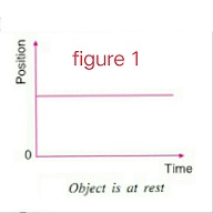
1. Position Time Graph When the Body is at Rest

Figure 1 shows the position-time graph when the body is at rest

The position-time graph for the stationary objects is a straight line parallel to the time axis.

2. Position Time Graph for Uniform Motion

Figure 2 shows a position time graph for uniform motion.

Here the object is moving along a straight line and covers equal distances in equal intervals of time.

3. Position Time Graph for an Object in Non-Uniform Motion

Figures 3 and 4 show a position-time graph for non-uniform motion.

In figure-3, acceleration is positive and in Figure-4, acceleration is negative.

Here, the object moves along a straight line and covers an equal distance in an unequal time interval.

II. Velocity Time Graph

The graph is plotted by taking time t along the x-axis and the velocity of the particle on the y-axis.

• The area of the velocity v/s time graph for the particular time interval gives the displacement and distance travelled by the body for a given time interval.

• The slope of the velocity-time graph represents the acceleration of the particle.

1. When a Particle is Moving With Constant Velocity

Figure 5 shows constant velocity and zero acceleration.

2. For Uniform Acceleration of the Particle

Figure 6 shows constant positive acceleration.

III. Acceleration-Time Graph

The graph is plotted by taking time t along the x-axis and the acceleration of the particle on the y-axis.

• The area of the acceleration v/s time graph for the particular time interval gives the change in velocity of the body for a given time interval.

• The slope of the acceleration-time graph represents the jerk.

1. When a Particle Has Constant Acceleration

Figure 7 represents uniform positive acceleration

2. A Particle having Uniformly Increasing Acceleration

Figure 8 represents positive and uniformly increasing acceleration.

Recommended Topic Video

Solved Examples based on kinematics Graph

Example 1: The velocity-displacement graph describing the motion of a bicycle is shown in the figure.

The acceleration-displacement graph of the bicycle's motion is best described by :

1)

2)

3)

4)

Solution:

$\begin{aligned} & \text { For } 0 \leq \mathrm{x} \leq 200 \\ & \mathrm{v}=\mathrm{mx}+\mathrm{C} \\ & \mathrm{v}=\frac{1}{5} \mathrm{x}+10 \\ & \mathrm{a}=\frac{\mathrm{vdv}}{\mathrm{dx}}=\left(\frac{\mathrm{x}}{5}+10\right)\left(\frac{1}{5}\right) \\ & \mathrm{a}=\frac{\mathrm{x}}{25}+2 \Rightarrow \text { Straight line till } \mathrm{x}=200 \\ & \text { for } x>200 \\ & v=\text { constant } \\ & \Rightarrow a=0\end{aligned}$

So the correct graph is

Hence the answer is the option (2)

Example 2: In the given position-time graph, which of the following is correct

1) I - Positive acceleration

II - Negative acceleration

III - Zero acceleration

2) I - Positive acceleration

II - Zero acceleration

III - Negative acceleration

3) All represent positive acceleration.

4) Nothing can be concluded

Solution:

I - Slope (i.e. velocity ) is increasing hence acceleration is positive.
II - Slope is constant $\Rightarrow a=0$
III - Slope is decreasing $\Rightarrow a<0$

Hence the answer is the option (2)

Example 3: Figure shows the displacement time graph of two particles moving along the x-axis. We can say that.

1) Both particles are having a uniformly retarded motion.

2) Both the particles have an accelerated motion.

3) Particle (1) is having an accelerated motion while particle (2) is having a retarding motion.

4) Particle (1) is having a retarded motion while particle (2) is having an accelerated motion.

Solution:

In graph (1), the slope i.e. velocity is continuously increasing and hence it depicts accelerated motion.

In graph (2), the slope i.e. velocity is continuously decreasing and hence it depicts retarding motion.

Hence the answer is the option (3)

Example 4: A particle is moving with constant velocity along a straight line. The position time graph will look like

1)

2)

3)

4)

Solution:

The slope of the Position-time graph represents the velocity. For a particle moving with non-zero constant velocity, the graph will be a straight line (constant slope).

Hence the answer is the option (2)

Example 5: A particle is stationary its position time graph will look like

1)

2)

3)

4)

Solution

Position time graph for a stationary object

The position-time graph for the stationary objects is a straight line parallel to the time axis.

wherein

shows the position-time graph of a stationary object.

Hence the answer is the option (4)

Summary

Kinematics graphs, including position-time, velocity-time, and acceleration-time graphs, are crucial for understanding the motion of objects. They visually represent various aspects of motion, such as velocity and acceleration, helping to analyze both uniform and non-uniform motion. These graphs are used to determine key motion characteristics, like displacement, acceleration, and velocity, and they provide valuable insights into different types of motion, whether the object is at rest, moving uniformly, or accelerating. Solved examples further illustrate the application of these graphs in analyzing real-life scenarios.