Solving Linear Equations Using Matrix

Solving linear equations is an important aspect of the algebra. Matrices offer a powerful formula to solve this equation more easily. These operations are applicable in real-life applications also. In real life, we use a Homogenous system of linear equations to solve the system of linear equations which helps us to solve age-related problems and time-related problems.

This Story also Contains

1. Matrix
2. Solving Linear Equations Using Matrix
3. Types of equation
4. Solved Examples Based on Solving Linear Equations Based on Matrices:

Matrix

A matrix (plural: matrices) is a rectangular arrangement of symbols along rows and columns that might be real or complex numbers. Thus, a system of $\mathrm{m} \times \mathrm{n}$ symbols arranged in a rectangular formation along m rows and n columns is called an $m$ by $n$ matrix (which is written as $\mathrm{m} \times \mathrm{n}$ matrix). The order of the matrix helps to get the numbers of rows and columns. The order helps us to understand the type of matrix and the total elements present in the matrix.

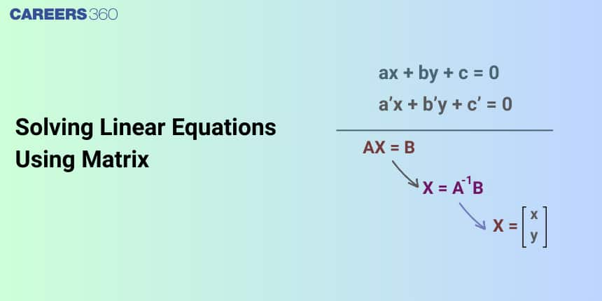
Solving Linear Equations Using Matrix

System of Linear Equation
A system of linear equations are group of $n$ linear equations containing $n$ number of variables.

1. System of 2 Linear Equations:

It is a pair of linear equations in two variables. It is usually of the form

$a_1x +b_1y + c_1 = 0$

$a_2x +b_2y + c_2 = 0$

Finding a solution for this system means finding the values of $x$ and $y$ that satisfy both equations.

2. System of 3 Linear Equations:

It is a group of 3 linear equations in three variables. It is usually of the form

$a_1x +b_1y + +c_1z + d_1 = 0$

$a_2x +b_2y + +c_2z + d_2 = 0$

$a_3x +b_3y + +c_3z + d_3 = 0$

Let us consider n linear equations in n unknowns, given as below
$
\begin{aligned}
& a_{11} x_1+a_{12} x_2+\ldots+a_{1 n} x_n=b_1 \\
& \mathrm{a}_{21} \mathrm{x}_1+\mathrm{a}_{22} \mathrm{x}_2+\ldots+\mathrm{a}_{2 \mathrm{n}} \mathrm{x}_{\mathrm{n}}=\mathrm{b}_2 \\
& \text {... } \qquad \text {... }\qquad \text {... }\qquad \text {... }\qquad \text {... }\\
& \text {... }\qquad \text {... } \qquad \text {... }\qquad \text {... }\qquad \text {... }\\
& \mathrm{a}_{\mathrm{n} 1} \mathrm{x}_1+\mathrm{a}_{\mathrm{n} 2} \mathrm{x}_2+\ldots+\mathrm{a}_{\mathrm{nn}} \mathrm{x}_{\mathrm{n}}=\mathrm{b}_{\mathrm{n}}
\end{aligned}
$

Here $\mathrm{x}_1, \mathrm{x}_2, \ldots \mathrm{x}_{\mathrm{n}}$ are n unknown variables
if $b_1=b_2=\ldots=b_n=0$ then the system of equation is known as the homogenous system of equation and if any of $b_1, b_2, \ldots b_n$ is non - zero then it is called non-homogenous system of equation

The above system of equations can be written in matrix form as

$
\begin{aligned}
& {\left[\begin{array}{ccccc}
a_{11} & a_{12} & \ldots & \ldots & a_{1 n} \\
a_{21} & a_{22} & \ldots & \ldots & a_{2 n} \\
\ldots & \ldots & \ldots & \ldots & \ldots \\
\ldots & \ldots & \ldots & \ldots & \ldots \\
a_{n 1} & a_{n 2} & \ldots & \ldots & a_{n n}
\end{array}\right]\left[\begin{array}{c}
x_1 \\
x_2 \\
\ldots \\
\ldots \\
x_n
\end{array}\right]=\left[\begin{array}{c}
b_1 \\
b_2 \\
\ldots \\
\ldots \\
b_n
\end{array}\right]} \\
& \Rightarrow \mathrm{AX}=\mathrm{B}, \text { where } \\
& \mathrm{A}=\left[\begin{array}{ccccc}
a_{11} & a_{12} & \ldots & \ldots & a_{1 n} \\
a_{21} & a_{22} & \ldots & \ldots & a_{2 n} \\
\ldots & \ldots & \ldots & \ldots & \ldots \\
\ldots & \ldots & \ldots & \ldots & \ldots \\
a_{n 1} & a_{n 2} & \ldots & \ldots & a_{n n}
\end{array}\right], \mathrm{X}=\left[\begin{array}{c}
x_1 \\
x_2 \\
\ldots \\
\ldots \\
x_n
\end{array}\right], \mathrm{B}=\left[\begin{array}{c}
b_1 \\
b_2 \\
\ldots \\
\ldots \\
b_n
\end{array}\right]
\end{aligned}
$

Premultiplying equation $A X=B$ by $A^{-1}$, we get

$\begin{aligned} A^{-1}(A X)= & A^{-1} B \Rightarrow\left(A^{-1} A\right) X=A^{-1} B \\ & \Rightarrow I X=A^{-1} B \\ & \Rightarrow X=A^{-1} B \\ & \Rightarrow X=\frac{\operatorname{adj} A}{|A|} B\end{aligned}$

Types of equation

1. The system of equations is non-homogenous:

   1. If $|A| \neq 0$, then the system of equations is consistent and has a unique solution $X=A^{-1} B$

   2. If $|A|=0$ and $(\operatorname{adj} A) \cdot B \neq 0$, then the system of equations is inconsistent and has no solution.

   3. If $|A|=0$ and $(\operatorname{adj} A) \cdot B=0$, then the system of equations is consistent and has an infinite number of solutions.

2. The system of equations is homogenous:

   1. If $|A| \neq 0$, then the system of equations has only one solution which is the trivial solution.

   2. If $|A|=0$, then the system of equations has the non-trivial solution and it has an infinite number of solutions.

Recommended Video Based on Solving Linear Equations Using Matrix:

Solved Examples Based on Solving Linear Equations Based on Matrices:

Example 1: The system of equations

$
\begin{aligned}
& x+y+z=6 \\
& x+2 y+3 z=14 \\
& x+4 y+7 z=30 \text { has }
\end{aligned}
$

1) no solution
2) unique solution
3) infinite solutions
4) none of these

Solution

We have

$
\begin{aligned}
& x+y+z=6 \\
& x+2 y+3 z=14 \\
& z+4 y+7 z=30
\end{aligned}
$
The given system of equations in the matrix form is written below:

$
\begin{aligned}
& {\left[\begin{array}{lll}
1 & 1 & 1 \\
1 & 2 & 3 \\
1 & 4 & 7
\end{array}\right]\left[\begin{array}{l}
x \\
y \\
z
\end{array}\right]=\left[\begin{array}{c}
6 \\
14 \\
30
\end{array}\right]} \\
& \mathrm{AX}=\mathrm{B} \quad \ldots .(1)
\end{aligned}
$
Where $\mathrm{A}=\left[\begin{array}{lll}1 & 1 & 1 \\ 1 & 2 & 3 \\ 1 & 4 & 7\end{array}\right], X=\left[\begin{array}{l}x \\ y \\ z\end{array}\right]$ and $B=\left[\begin{array}{c}6 \\ 14 \\ 30\end{array}\right]$

$
\begin{aligned}
|\mathrm{A}| & =1(14-12)-1(7-3)+1(4-2) \\
& =2-4+2=0
\end{aligned}
$

$\therefore$ The equation either has no solution or an infinite number of solutions.
To decide about this, we need to find $\operatorname{adj}(A)$. $B$

On comparing

$
x+y+z=6, y+2 z=8
$
Taking $z=k \in R$

$
\begin{array}{ll}
\therefore & y=8-2 k \\
\text { and } & x=k-2
\end{array}
$
Since k is arbitrary, hence the number of solutions is infinite.
Hence, the answer is option 3.

Example 2: Solve the system of equations

$
\begin{aligned}
& x+y+z=6 \\
& x+2 y+3 z=14 \\
& x+4 y+7 z=30 \text { has }
\end{aligned}
$

1) no solution
2) unique solution
3 ) infinite solutions
4) none of these

Solution

As we have learned
Non-homogeneous system of linear equation -

$
b \neq 0
$

- wherein

Given system of equation is

$
\begin{aligned}
& x+y+z=6 \\
& x+2 y+3 z=14 \\
& x+4 y+7 z=30
\end{aligned}
$

$\begin{aligned} & \Delta=\left|\begin{array}{lll}1 & 1 & 1 \\ 1 & 2 & 3 \\ 1 & 4 & 7\end{array}\right|=1(14-12)-1(7-3)+1(4-2)=0 \\ & \Delta_1=\left|\begin{array}{lll}6 & 1 & 1 \\ 14 & 2 & 3 \\ 30 & 4 & 7\end{array}\right|=0 \\ & \Delta_2=\left|\begin{array}{lll}1 & 6 & 1 \\ 1 & 14 & 3 \\ 1 & 30 & 7\end{array}\right|=0 \\ & \Delta_3=\left|\begin{array}{lll}1 & 1 & 6 \\ 1 & 2 & 14 \\ 1 & 4 & 30\end{array}\right|=0\end{aligned}$

Aso,

$
\begin{aligned}
& x+y+z=6 \ldots(1) \\
& y+2 z=8 \ldots(2) \\
& x=6-y-z=6-(8-2 z)-z=z-2
\end{aligned}
$
Taking $z=k$, we get $x=k-2, y=8-2 k ; k \in R$
Putting $\mathrm{k}=1$, we have one solution as $\mathrm{x}=-1, \mathrm{y}=6, \mathrm{z}=1$.
Thus by giving different values for k we get different solutions.
Hence the given system has an infinite number of solutions.

Example 3: If the system of linear equations

$
\begin{aligned}
& 2 x+2 y+3 z=a \\
& 3 x-y+5 z=b \\
& x-3 y+2 z=c
\end{aligned}
$

where $a, b, c$ are non-zero real numbers, has more than one solution, then :
1) $b-c-a=0$
2) $b+c-a=0$
3) $b-c+a=0$
4) $a+b+c=0$

Solution

Solution of a system of equations -
$x_1, x_2, \cdots, x_n$ satisfy the system of linear equations $A x=B$
- wherein

For these 3 equations having more than 1 solution

$
\begin{aligned}
& \Rightarrow D=0 \\
& \Rightarrow\left|\begin{array}{ccc}
2 & 2 & 3 \\
3 & -1 & 5 \\
1 & -3 & 2
\end{array}\right|=0 \\
& \Rightarrow 26-20-24=0 \\
& \Rightarrow D=0
\end{aligned}
$
Also, $D_1=D_2=D_3=0$

$
\begin{aligned}
& D_1=\left|\begin{array}{ccc}
a & 2 & 3 \\
b & -1 & 5 \\
c & -3 & 2
\end{array}\right|=0 \\
& \Rightarrow a(13)-b(13)+c(13)=0 \\
& \Rightarrow a-b+c=0
\end{aligned}
$

$\begin{aligned} & D_2=0 \Rightarrow\left|\begin{array}{ccc}2 & a & 3 \\ 3 & b & 5 \\ 1 & c & 2\end{array}\right|=0 \\ & \Rightarrow a-b+c=0 \\ & D_3=0 \Rightarrow\left|\begin{array}{ccc}2 & 2 & a \\ 3 & -1 & b \\ -1 & -3 & c\end{array}\right|=0 \\ & \Rightarrow a-b+c=0\end{aligned}$

Example 4:If $A=\left[\begin{array}{lll}1 & 2 & x \\ 3 & -1 & 2\end{array}\right]$ and $\mathrm{B}=\left[\begin{array}{l}y \\ x \\ 1\end{array}\right]$ such that $\mathrm{AB}=\left[\begin{array}{l}6 \\ 8\end{array}\right]$ then:

1) $y=2 x$
2) $y=-2 x$
3) $y=x$
4) $y=-x$

Solution

As we learnt in

Solution of a non-homogeneous system of linear equations by matrix method -

If $A$ is a non-singular matrix then the system of equations given by $A x=b$ has a unique solution given by $x=A^{-1} b$

$
\begin{aligned}
& \text { - wherein } \\
& A=\left[\begin{array}{ccc}
1 & 2 & x \\
3 & -1 & 2
\end{array}\right] \\
& B=\left[\begin{array}{l}
y \\
x \\
1
\end{array}\right] \\
& A B=\left[\begin{array}{l}
6 \\
8
\end{array}\right] \\
& \therefore\left[\begin{array}{ccc}
1 & 2 & x \\
3 & -1 & 2
\end{array}\right]\left[\begin{array}{l}
y \\
x \\
1
\end{array}\right]=\left[\begin{array}{l}
6 \\
8
\end{array}\right] \\
& =\left[\begin{array}{l}
y+2 x+x \\
3 y-x+2
\end{array}\right]=\left[\begin{array}{l}
6 \\
8
\end{array}\right] \\
& \Rightarrow y+3 x=6 \\
& -x+3 y=6
\end{aligned}
$
So, $y+3 x=-x+3 y$

$
\begin{aligned}
& \Rightarrow 4 x=2 y \\
& \therefore y=2 x
\end{aligned}
$
Example 5: An ordered pair $(\alpha, \beta)$ for which the system of linear equations

$
\begin{aligned}
& (1+\alpha) x+\beta y+z=2 \\
& \alpha x+(1+\beta) y+z=3 \\
& \alpha x+\beta y+2 z=2
\end{aligned}
$

has a unique solution, is:

1) $(2,4)$
2) $(-4,2)$
3) $(1,-3)$
4) $(-3,1)$

Solution

$
\begin{aligned}
& (1+\alpha) x+\beta y+z=0 \\
& \alpha x+(1+\beta) y+z=0 \\
& \alpha x+\beta y+2 z=0 \\
& D=\left|\begin{array}{ccc}
1+\alpha & \beta & 1 \\
\alpha & 1+\beta & 1 \\
\alpha & \beta & 2
\end{array}\right| \\
& C_1 \rightarrow C_1+C_2+C_3 \\
& D=(\alpha+\beta+2)\left|\begin{array}{ccc}
1 & \beta & 1 \\
1 & 1+\beta & 1 \\
1 & \beta & 2
\end{array}\right| \\
& R_2 \rightarrow R_2-R_1 \quad R_3 \rightarrow R_3-R_1 \\
& D=(\alpha+\beta+2)\left|\begin{array}{ccc}
1 & \beta & 1 \\
0 & 1 & 0 \\
0 & 0 & 1
\end{array}\right|=\alpha+\beta+2
\end{aligned}
$
For a unique solution, $\alpha+\beta \neq-2$